Evaluating Topic Models - In Practice
Having already talked about why it’s hard to evaluate topic models, I wanted to walk through how I’ve ended up evaluating topic models when I’ve made them myself. This is from a project I’m still working on and I’m not sure it’s ethical for me to share the data, but the code can be easily repurposed. I’ll share the link to an ipynb with all of the code I used.
Caveat
This is all done with SKLearn’s LDA implementation so it goes without saying that you can’t just plug this all into say Gensim’s approach and use it without any modification.
Warning(s)
This is an incredibly slow process. Don’t expect it to be fast, especially on larger data. You have been warned.
Because this is from a personal project where I have to keep the data private, I can’t share the data. Thus, you can’t follow along with me. I’m planning on finding (or making) a good public dataset that I write another post about so you can follow along.
Starting with the first imports and why
import pandas as pd
import numpy as np
from sklearn.decomposition import LatentDirichletAllocation
from sklearn.feature_extraction.text import TfidfVectorizer, CountVectorizer
We’re using Pandas as the wrapper for the handling the data. We’re bringing Numpy to be safe because I believe it’s better to have it than not. Then we’ve got the SKLearn LDA and vectorizers.
The horribly messy pre-processing step
import string
punct = string.punctuation
punct = punct.replace("#", "‘")
 #removing hashtag and replacing with a stray type of apostrophe that broke through

import nltk
from nltk.stem import WordNetLemmatizer
wordnet_lemmatizer = WordNetLemmatizer()
stopwords = nltk.corpus.stopwords.words("english")
import contractions

# defining a pre-proc function that will tokenize text
def pre_proc(x):
    # splitting contractions before splitting up the terms => helps with pruning
    # trying to expand the contractions
    try:
        x = contractions.fix(x)

    # if that fails, trying to use unidecode to correct
    except IndexError:
        # trying to unidecode
        try:
            x = contractions.fix(unidecode(x))

        except Exception as eror: # printing excpetion, and input leading to that
            print("Exception is:", error)
            print("Exception on:")
            print(x)

    x = x.split() # splitting the terms up

    x = [word for word in x if len(word)>0] # removing the empty items

    x = [word.lower() for word in x] # lowercasing the terms

    # removing emoji & conveniently, some punctuation
    x = [word.encode("ascii", "ignore").decode("ascii") for word in x]

    # removing punctuation (with the exception of #)
    x = [word.translate(str.maketrans("","",punct)) for word in x]


    x = [word for word in x if len(word)>0] # removing the empty items

    x = [word for word in x if word not in stopwords]     # removing stopwords

    x = [wordnet_lemmatizer.lemmatize(word) for word in x]     # lemmatization

    x = " ".join(x)      # rejoining the list back into a string

    return x
This is kinda messy but it’s what I’ve used on multiple occasions. It works for my purposes here and it worked in my masters paper. The main thing to note is we want to return a string that has been cleaned because that’s what it takes to ensure some of the metrics work properly.
Running the pre-processing, reading data, vectorizing
chapters = pd.read_json("book_chapters.jl", lines=True) # reading data

chapters["clean"] = chapters["chapt_text"].apply(pre_proc)

tf_vectorizer = CountVectorizer(
    max_df=0.95, min_df=.1, stop_words="english"
)

tf = tf_vectorizer.fit_transform(chapters["clean"])
Setting everything up to search for optimal K
k_vals = [3, 6, 9, 12, 15, 18, 21, 25, 30, 35, 40] # decent spread of k-vals

# making lists to hold the scores for each of these topic model values
perp_scores = list()
ll_scores =list()
silh_scores = list()
ch_scores = list()
coh_umass_scores = list()
coh_c_v_scores = list()
coh_c_uci_scores = list()
coh_c_npmi_scores = list()

tokens = chapters["clean"].apply(str.split) # we need this for one of the metrics

import time # we need this to ensure we have all the timings
Running multiple LDA models and getting the metrics for search
# importing our metrics
from sklearn.metrics import silhouette_score
from sklearn.metrics import calinski_harabasz_score
from tmtoolkit.topicmod.evaluate import metric_coherence_gensim


start_time = time.time()  #timing is everything

for k in k_vals:
    loop_start = time.time()
    lda = LatentDirichletAllocation(n_components=k, random_state=0, n_jobs=5) # making our lda model

    lda.fit(tf) # fitting it to our tf

    # getting our labels for the silhouette score and CH
    labels = lda.transform(tf)
    doc_labels = [label.argmax() for label in labels] # list comp which gives labels for each doc

    # getting our metrics next
    perp_scores.append(lda.perplexity(tf))
    ll_scores.append(lda.score(tf))
    silh_scores.append(silhouette_score(tf, doc_labels))
    ch_scores.append(calinski_harabasz_score(tf.toarray(), doc_labels))

    # coherence scores
    coh_umass_scores.append(metric_coherence_gensim(measure='u_mass', # the measure we're using
                        top_n=25,
                        topic_word_distrib=lda.components_, # the components of the lda count as
                        dtm=tf, # the term frequency
                        vocab=np.array([x for x in tf_vectorizer.vocabulary_.keys()]), # pass in vectorizer
                        texts=tokens, # pass in list of tokenized texts -> needs to match vocab -> if using umass, doesn't matter at all
                        return_mean=True)) # return the mean coherence score for the model

    coh_c_v_scores.append(metric_coherence_gensim(measure='c_v', # the measure we're using
                        top_n=25,
                        topic_word_distrib=lda.components_, # the components of the lda count as
                        dtm=tf, # the term frequency
                        vocab=np.array([x for x in tf_vectorizer.vocabulary_.keys()]), # pass in vectorizer
                        texts=tokens, # pass in list of tokenized texts -> needs to match vocab -> if using umass, doesn't matter at all
                        return_mean=True))

    coh_c_uci_scores.append(metric_coherence_gensim(measure='c_uci', # the measure we're using
                        top_n=25,
                        topic_word_distrib=lda.components_, # the components of the lda count as
                        dtm=tf, # the term frequency
                        vocab=np.array([x for x in tf_vectorizer.vocabulary_.keys()]), # pass in vectorizer
                        texts=tokens, # pass in list of tokenized texts -> needs to match vocab -> if using umass, doesn't matter at all
                        return_mean=True))

    coh_c_npmi_scores.append(metric_coherence_gensim(measure='c_npmi', # the measure we're using
                        top_n=25,
                        topic_word_distrib=lda.components_, # the components of the lda count as
                        dtm=tf, # the term frequency
                        vocab=np.array([x for x in tf_vectorizer.vocabulary_.keys()]), # pass in vectorizer
                        texts=tokens, # pass in list of tokenized texts -> needs to match vocab -> if using umass, doesn't matter at all
                        return_mean=True))


    loop_end = time.time()
    print("loop took", loop_end - loop_start, "seconds to run")
end_time = time.time()

print("total time", end_time - start_time, "seconds")
I know that’s a bit messy and my comments mean that it doesn’t all fit on there, but the gist is we’re going through and grabbing the metrics for each time we build an LDA topic model.
Comparing the results
import matplotlib.pyplot as plt

plt.rcParams['figure.dpi'] = 150 # ensuring we have a good size for vectorizers

fig, axs = plt.subplots(4, 2)
fig.suptitle("Metrics vs. K")
fig.tight_layout(pad=1.5)


axs[0,0].plot(k_vals, perp_scores, "blue", label="perplexity")
axs[0,0].set_title("perplexity")

axs[0,1].plot(k_vals, ll_scores, "red", label="log likliehood")
axs[0,1].set_title("log likliehood")

axs[1,0].plot(k_vals, silh_scores, "Orange" , label= "silhouette score")
axs[1,0].set_title("silhouette score")

axs[1,1].plot(k_vals, ch_scores, "Yellow", label="CH score")
axs[1,1].set_title("CH score")

axs[2,0].plot(k_vals, coh_umass_scores, "Green", label="Coh UMass")
axs[2,0].set_title("Coh UMass")

axs[2,1].plot(k_vals, coh_c_v_scores, "Purple", label="Coh C_V")
axs[2,1].set_title("Coh C_V")

axs[3,0].plot(k_vals, coh_c_uci_scores, "Pink", label="Coh C_UCI")
axs[3,0].set_title("Coh C_UCI")

axs[3,1].plot(k_vals, coh_c_npmi_scores, "magenta", label="Coh C_NPMI")
axs[3,1].set_title("Coh C_NPMI")
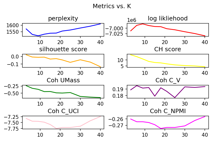
Lower Perplexity scores are better while higher log likliehood is better. From these, it would seem like the better value for K is somewhere around 10. Of course, we have other metrics as well to examine. For silhouette score, the closer to 1 the better it is. Thus, it would seem that we want to have a value below 10. For CH Score, the higher it is the better so again, we seem to want to aim for lower than 10 topics.
Pivoting to Coherence, the goal is to maximize the coherence value. Thus, again, we see hints that we want to stick with fewer than 10 topics or alternatively go far beyond 10 topics (somewhere between 30 and 40 topics perhaps for 3 coherence metrics).
We can always optimize further if we have the time and compute resources to do so. Since this is a fairly small set of data, we can go ahead and do so. In this case, I did so in the ipynb, but I’m not going to make you go through that.
Tuning Parameters
One thing I did in the ipynb that I won’t do here is I worked to tune the hyperparameters. That didn’t make much of a difference at all so that’s why I’m leaving it be here.
PyLDAvis Visualization
The final step once you’ve got some good candidates is to check them with PyLDAvis. You want to start by taking your candidate values in terms of hyperparameters and combine those with the k value(s) you determined are worth exploring. You then make some lda models and feed those into pyLDAvis. PyLDAvis can help you by letting you visually see how the topics fit together. You do this for each candidate parameter set.
cand_vals = [(.1, .05),(.5, 1), (1, .75), (1,1)] # these are my best guess for where we see those spikes

import pyLDAvis.sklearn

lda1 = LatentDirichletAllocation(n_components=k, random_state=0, n_jobs=5,
                           doc_topic_prior=cand_vals[0][0],
                           topic_word_prior=cand_vals[0][1]) # making our lda model (w/hyper-params)
lda1.fit(tf)

pyLDAvis.enable_notebook()
lda1_dash = pyLDAvis.sklearn.prepare(lda1, tf, tf_vectorizer)
lda1_dash
In my case, I saw that there were two topics that had overlap. The solution there is to adjust the number of topics down by the number of overlapping topics. In this case for me, I adjusted the K down to 7. Sadly, the result of PyLDAvis doesn’t lend itself to static imagery or I would include another picture. Hopefully, this gives a better idea of how to approach optimizing your K value. I’m thinking I may go ahead and redo this exercise with a public dataset so y’all can follow along.